Residual-based a posteriori error estimates with boundary correction for φ-FEM
The φ-Finite Element Method
The φ-FEM belongs to the family of Immersed Boundary Methods. It is designed to solve partial differential equations (PDEs) on complicated domains with unfitted meshes.

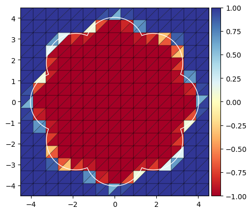
On the above figure, the exact domain is delimited by the “flower-shaped” white curve. In φ-FEM, a PDE can be solved on this domain using the unfitted mesh (called background mesh) shown on the figure.
What sets φ-FEM apart from other Immersed Boundary Methods is that there is no integral to compute on cut elements, so no unconventional quadrature rule is needed.
Let \(\varphi\) be a sufficiently regular levelset function. The physical domain \(\Omega\) and its boundary \(\Gamma\) are defined via \(\varphi\) as follow
\[\begin{equation} \Omega := \{\varphi < 0\},\quad \Gamma := \{\varphi = 0\}. \end{equation}\]Thus, given \(f \in L^2(\Omega)\), we are interested by the following Poisson–Dirichlet problem: seek \(u\) such that
\[\begin{equation} -\Delta u = f\quad \text{in } \Omega,\qquad u = 0\quad \text{on } \Gamma. \end{equation}\]The key idea of φ-FEM is to reformulate the function \(u\) as: \(\varphi w\) and to approximate this product by \(\varphi_h w_h\), where \(\varphi_h\) is an interpolation of \(\varphi\) on the background mesh and \(w_h\) is a finite element function also defined on the background mesh.
Let us denote \(\mathcal T_h^{\mathcal O}\) the background mesh, \(\mathcal T_h := \{T \in \mathcal T_h^{\mathcal O};\ T \cap \{\varphi_h < 0\} \neq \varnothing\}\) and \(\Omega_h := \cup_{T \in \mathcal T_h} T\). We introduce the linear Lagrange finite element space
\[\begin{equation} V_h := \left\{v_h \in H^1(\Omega);\ {v_h}_{|T} \in \mathbb P_1(T)\ \forall T \in \mathcal T_h \right\}. \end{equation}\]Remark: For the sake of simplicity we consider a linear Lagrange space only but stress out that φ-FEM can be straightforwardly extended to higher order spaces.
The function \(w_h\) is taken as the solution to the following φ-FEM discrete formulation: for all \(v_h \in V_h\),
\[\begin{equation} \int_{\Omega_h} \nabla \varphi_h w_h \cdot \nabla \varphi_h v_h + \int_{\partial \Omega_h} \frac{\partial}{\partial } (\varphi_h w_h) \varphi_h v_h + G_h(w_h, v_h) = \int_{\Omega_h} f \varphi_h v_h + G_h^{\mathrm{rhs}}(v_h), \end{equation}\]where \(G_h\) and \(G_h^{\mathrm{rhs}}\) are stabilization terms (see the original publication for the definitions).
A residual-based error estimator
Given the φ-FEM solution \(u_h = \varphi_h w_h\), we can derive the following a posteriori error estimator:
\[\begin{equation} \eta^2 := \sum_{T \in \mathcal T_h} \eta_T^2,\quad \text{where}\quad \eta_T^2 := \eta_{r, T}^2 + \eta_{J, T}^2 + \eta_{\varepsilon, T}^2, \end{equation}\]and
\[\begin{align} \eta_{r,T} &:= h_T \| f_h + \Delta u_h\|_{L^2(T)},\\ \eta_{J,T} &:= \frac{1}{2} \left[ \sum_{E \in \partial T} h_E \left\|\left[\frac{\partial}{\partial n} u_h \right]_E \right\|_{L^2(E)}^2\right]^{1/2},\\ \eta_{\varepsilon,T} &:= |\varepsilon_h|_{H^1(T)}. \end{align}\]Remark: For a cell \(T\), the terms \(\eta_{r,T}\) and \(\eta_{J,T}\) are similar to the terms in the residual estimator for a standard FEM discretization of the Poisson-Dirichlet equation.
We show the reliability of \(\eta\), in other words, there exists a constant \(C\) depending on the regularity of the mesh only such that
\[\begin{equation} \lvert u - u_h \rvert_{H^1(\Omega)} \leqslant C \eta + \mathrm{h.o.t.}, \label{eq:reliability} \end{equation}\]where \(\mathrm{h.o.t.}\) are higher order terms, composed of oscillation terms from the discretization of \(f\) and of \(\varphi\).
The boundary correction term
Let us detail why the boundary correction term, namely \(\eta_{\varepsilon, T}\), is essential to the proof of eq. \((\ref{eq:reliability})\). This correction term trick has been introduced for the first time in here in the context of a cutFEM.
To explain properly where does this term come from, let us first recall the proof of the reliability of the standard residual estimator. Assume for a moment that the domain \(\mathcal T_h\) fits the domain \(\Omega\) and that \(u_h^*\) is the solution of the finite element problem
\[\begin{equation} \int_{\Omega} \nabla u_h^* \cdot \nabla v_h = \int_{\Omega} f v_h\quad \forall v_h \in V_h^*, \end{equation}\]where \(V_h^*\) is the subset of \(V_h\) of functions vanishing on \(\Gamma\). Then \(u_h^* \in H^1_0(\Omega)\) and so is \(u - u_h^*\). Moreover, we have Galerkin orthogonality: \(u - u_h^*\) is orthogonal to \(V_h^*\) in \(H^1_0(\Omega)\). Thus, for any \(v \in H^1_0(\Omega)\), if we denote \(\mathcal I_h v\) its Lagrange interpolant to \(V_h^*\), we have
\[\begin{equation} \int_{\Omega} \nabla (u - u_h^*) \cdot \nabla v = \int_{\Omega} f (v - \mathcal I_h v) - \int_{\Omega} \nabla u_h^* \cdot \nabla (v - \mathcal I_h v), \label{eq:galerkin} \end{equation}\]the interpolant being introduced thanks to Galerkin orthogonality.
Now all the key pieces are in place and the remaining steps are:
1) Apply a cellwise integration by parts on the last integral of eq. \((\ref{eq:galerkin})\),
2) Apply standard inequalities (Cauchy-Schwarz, trace and interpolation),
3) Recall that
\(\begin{equation} \lvert u - u_h^* \rvert_{H^1(\Omega)} = \underset{v \in H^1_0(\Omega), \lvert v \rvert \neq 0}{\min} \frac{\displaystyle \int_{\Omega} \nabla (u - u_h^*) \cdot \nabla v}{\displaystyle \lvert v \rvert_{H^1(\Omega)}} \end{equation}\),
4) If everything went well, on the right hand side you would be able to get \((\eta + \mathrm{h.o.t.}) \lvert v \rvert_{H^1(\Omega)}\),
In this proof, one of the key ingredients is that \(u - u_h^*\) belongs to \(H^1_0(\Omega)\),
Now, let us come back to our φ-FEM case. If we consider \(u - u_h\), we remark that this function does not belong to \(H^1_0(\Omega)\). This is where \(\varepsilon\) and its discretization \(\varepsilon_h\) come into play: we decompose \(u - u_h\) as a part in \(H^1_0(\Omega)\) and a part orthogonal to \(H^1_0(\Omega)\), denote \(\varepsilon\).
The first step of the proof of eq. \((\ref{eq:reliability})\) consists in the introdution of a proper \(\varepsilon\) function. Let us consider \(\Pi u_h\) the solution to
\[\begin{equation} \int_{\Omega} \nabla \Pi u_h \cdot \nabla v = \int_{\Omega} \nabla u_h \cdot \nabla v\quad \forall v \in H^1_0(\Omega). \end{equation}\]In other words, \(\Pi u_h\) is the orthogonal projection of \(u_h\) onto \(H^1_0(\Omega)\) with respect to the \(H^1_0(\Omega)\) inner product.
Now let us define \(\varepsilon := \Pi u_h - u_h\). Thus, \(\varepsilon\) is orthogonal to \(H^1_0(\Omega)\), which yields
\[\begin{equation} \lvert u - u_h \vert_{H^1(\Omega)} = \lvert u - \Pi u_h \rvert_{H^1(\Omega)} + \lvert \Pi u_h - u_h \rvert_{H^1(\Omega)}, \label{eq:orthogonality} \end{equation}\]since \(u - \Pi u_h \in H^1_0(\Omega)\).
The second term of the right hand side of eq. \((\ref{eq:orthogonality})\) is \(\lvert \varepsilon \rvert_{H^1(\Omega)}\) which is not computable as such, since \(\Pi u_h\) is not a discrete function. Therefore, we introduce
\[\begin{align} \lvert \varepsilon \rvert_{H^1(\Omega)} &= \lvert \Pi u_h - u_h \rvert_{H^1(\Omega)}\notag\\ &= \underset{v \in H^1_0(\Omega)}{\min} \lvert v - \varphi_h w_h \rvert_{H^1(\Omega)}\notag\\ &\leqslant \lvert \varphi w_h - \varphi_h w_h \rvert_{H^1(\Omega)}\notag\\ &\approx \lvert (\widetilde \varphi_h - \varphi_h) w_h \rvert_{H^1(\Omega)} =: \lvert \varepsilon_h \rvert_{H^1(\Omega)} \end{align}\]where \(\widetilde \varphi_h\) is a finer approximation of \(\varphi\) (e.g. its interpolation into a higher degree Lagrange finite element space).
Remark: The function \(\varepsilon_h\) can be see as a hierarchical approximation of the boundary discretization error induced by the interpolation \(\varphi_h\). This term can be constructed such that it vanishes inside \(\Omega\), far away from \(\Gamma\). Then, only its values around \(\Gamma\) influence the estimator \(\eta\).
Using a triangular inequality in eq. \((\ref{eq:orthogonality})\) we obtain
\[\begin{equation} \lvert u - u_h \vert_{H^1(\Omega)} \leqslant \lvert u - \Pi u_h \rvert_{H^1(\Omega)} + \lvert \varepsilon_h \rvert_{H^1(\Omega)} + \lvert \varepsilon - \varepsilon_h \rvert_{H^1(\Omega)}, \label{eq:epsilon_oscillations} \end{equation}\]where \(\lvert \varepsilon - \varepsilon_h \rvert_{H^1(\Omega)}\) can be proven to be of higher order and where \(\lvert \varepsilon_h \rvert_{H^1(\Omega)}\) can be decomposed as a sum of local contributions, leading to \(\eta_{\varepsilon, T}\).
Remark: The first term on the right hand side of eq. \((\ref{eq:epsilon_oscillations})\) can be controlled using the same tools as for the standard residual estimator, except two important points:
- at some point a Hardy type inequality is necessary, see Lemma 6 here,
- due to the discrepancy between \(\Gamma\) and \(\{\varphi_h = 0\}\) (the exact boundary and its approximation), we have to assume that \(f_h\) is the \(L^2\) projection of \(f\) onto \(V_h\), which is not what is usually required in the standard case. In practice, for the sake of computational cost, \(f_h\) is always taken as the interpolation of \(f\) onto \(V_h\) (or sometimes even onto a coarser space), therefore it might be possible to further improve the proof of eq. \((\ref{eq:reliability})\).
An adaptive φ-FEM
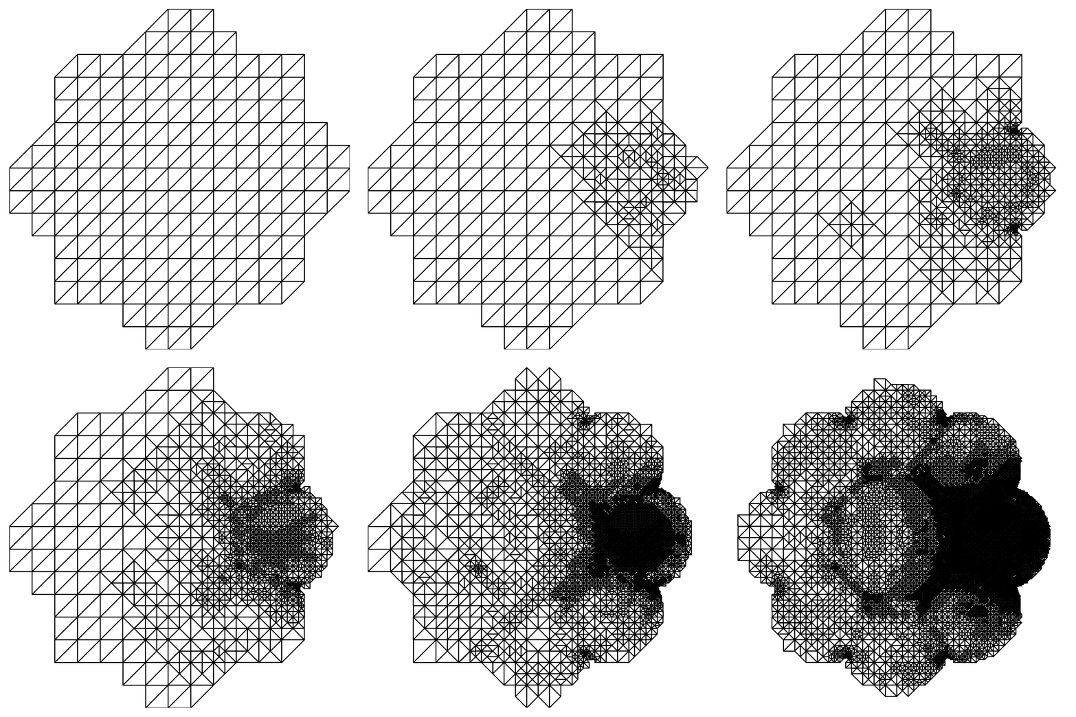
This novel estimator allows to derive an adaptive mesh refinement loop:
\[\begin{equation*} \cdots \longrightarrow \mathrm{SOLVE} \longrightarrow \mathrm{ESTIMATE} \longrightarrow \mathrm{MARK} \longrightarrow \mathrm{REFINE} \longrightarrow \cdots \end{equation*}\]Here is an example on the “flower-shaped” domain with a piecewise constant source term equal to 10 in a circular region on the right of the domain and 0 elsewhere.
Remarks:
- Note the extra refinement at the several reentrant corners of the domain, this is expected due to singular gradients of the solution \(u\) at these points.
- On the last mesh, we can see a circle of refinement in the middle of the domain, this shouldn’t be there. It appears because we are using a non-smooth levelset function \(\varphi\) in this numerical example. With a smooth \(\varphi\) only refinement on the right region and refinement near the reentrant corners should appear.
